Differentiation

강좌: 수치해석

Finite Difference

Taylor expansion 을 이용하면 수치 미분을 구할 수 있다.

First-order derivative

Fig. 20 Finite Difference (from Wikipedia)

• Forward Difference

\[ f'(x_j) = \frac{f(x_{j+1}) - f(x_j)}{\Delta x} + O(\Delta x) \approx \frac{\Delta f(x)}{\Delta x} \]

• Backward Differnce

\[ f'(x_j) = \frac{f(x_{j}) - f(x_{j-1})}{\Delta x} + O(\Delta x) \approx \frac{\nabla f(x)}{\Delta x} \]

• Central Difference

  • 다음 두 식을 빼보자.

\[ f(x_{j+1}) = f(x_j) + \Delta x f'(x_j) + \frac{(\Delta x)^2}{2} f''(x_j) + \frac{(\Delta x)^3}{3!} f'''(x_j) + O((\Delta x)^2) \]

\[ f(x_{j-1}) = f(x_j) - \Delta x f'(x_j) + \frac{(\Delta x)^2}{2} f''(x_j) - \frac{(\Delta x)^3}{3!} f'''(x_j) + O((\Delta x)^3) \]

• 그 결과는 다음과 같다.

\[ f'(x_j) = \frac{f(x_{j+1}) - f(x_{j-1})}{ 2\Delta x} + O((\Delta x)^2) \approx \frac{\delta f(x)}{2 \Delta x} \]

Second-order derivative

• Central Difference

  • 위의 두 식을 더한 후 \(2 f(x_j)\) 를 빼보자.

\[ f''(x_j) = \frac{f(x_{j+1}) + 2 f(x_j) - f(x_{j-1})}{ (\Delta x)^2} + O((\Delta x)^2) \]

제차분식

• Second-order Central

  \[ f''(x) \approx \frac{\delta^2 f(x) }{ (\Delta x)^2} = \frac{\Delta f(x) - \nabla f(x) }{\Delta x} = \frac{f(x_{j+1}) + 2 f(x_j) - f(x_{j-1})}{ (\Delta x)^2} \]

  • \(E=O((\Delta x)^2)\)

• Second-order Forward

  \[ f''(x) \approx \frac{\Delta^2 f(x) }{ (\Delta x)^2} = \frac{\Delta f(x+\Delta x) - \Delta f(x) }{\Delta x} = \frac{f(x_{j+2}) - 2 f(x_{j+1}) + f(x_{j})}{ (\Delta x)^2} \]

  • \(E=O((\Delta x))\)

• Second-order Backward

  \[ f''(x) \approx \frac{\nabla^2 f(x) }{ (\Delta x)^2} = \frac{\nabla f(x) - \nabla f(x - \Delta x) }{\Delta x} = \frac{f(x_{j}) - 2 f(x_{j-1}) + f(x_{j-2})}{ (\Delta x)^2} \]

  • \(E=O((\Delta x))\)

General approaches

• 일반적인 방법

  • 여러 Taylor expansion의 합차를 이용해서 원하는 미분항의 근사식을 구한다.

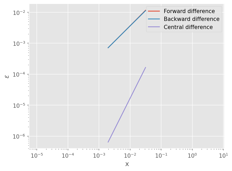
예제

\(f(x)=\sin(x)\) 에 대해서 수치 미분 결과를 비교하자.

%matplotlib inline
from matplotlib import pyplot as plt

import numpy as np

plt.style.use('ggplot')
plt.rcParams['figure.dpi'] = 150

x = 0.2*np.pi
dx = 0.01*np.pi
f = np.sin

# First-order forward 
fdf = (f(x+dx) - f(x)) / dx

# First-order backward
bdf = (f(x) - f(x-dx)) / dx

# First-order central
cdf = (f(x+dx) - f(x-dx)) / (2*dx)

print("Exact: ", np.cos(x))
print(fdf, bdf, cdf)

Exact:  0.8090169943749475
0.7996517731793618 0.8181160727815516 0.8088839229804567

# Exact difference
df = np.cos(x)

# Reducing dx and confirm errors
dxs = [0.01*np.pi, 0.005*np.pi, 0.0025*np.pi, 0.00125*np.pi, 0.000625*np.pi]

# Fowrad difference
err_fw = []
for dx in dxs:
    fdf = (f(x+dx) - f(x)) / dx
    err_fw.append(abs((fdf -df)/df))
    
# Backward difference
err_bw = []
for dx in dxs:
    bdf = (f(x) - f(x-dx)) / dx
    err_bw.append(abs((bdf -df)/df))    
    
# Central difference
err_ct = []
for dx in dxs:
    cdf = (f(x+dx) - f(x-dx)) / (2*dx)
    err_ct.append(abs((cdf -df)/df))       
    
# Plot log-log graph    
plt.loglog(dxs, err_fw)
plt.loglog(dxs, err_bw)
plt.loglog(dxs, err_ct)

# Same scale of x and y
plt.axis('equal')

# Legend
plt.legend([
    'Forward difference',
    'Backward difference',
    'Central difference',
])

plt.xlabel('x')
plt.ylabel('$\epsilon$')

Text(0, 0.5, '$\\epsilon$')